From Lab Bench to Browser: A Hybrid Digital Twin for CHO Cell Culture

Richelle et al. (2025) (bioRxiv 2025.11.24.690194)
GEM reduction pipeline from Antonakoudis & Richelle (2026) (npj Systems Biology and Applications)

If you’ve ever run a CHO fed-batch, you know the loop: set your conditions, feed your boluses, pull samples for two weeks, and find out at the end whether the run did what you hoped. The space of things you’d like to know about that culture is enormous. The number of experiments you can actually afford to run is not. That gap is the whole reason mechanistic models and digital twins exist, and it’s the reason I built this one.

Thank you for reading this post, don't forget to subscribe!

What follows is a tour of an interactive CHO digital twin I put together: a hybrid mechanistic-plus-machine-learning model, a genome-scale metabolic network reduction pipeline, and a web app that wraps the whole thing so you can poke at it without touching a flask. It’s a faithful, equation-by-equation replication of two recent papers, with my own engineering on top to make it run live in a browser.

One thing up front, so nobody goes hunting: there’s no hosted version online right now. The full source is on GitHub and you can run it locally today. I’ll put a public instance up soon, and I’ll update this post with the URL when it’s live.

The problem I’m actually trying to solve

Monoclonal antibodies, recombinant proteins, vaccines — most of the biologics that have reshaped oncology, immunology and infectious disease over the last thirty years are made the same way: inside a living cell, in a stirred tank, fed a carefully tuned nutrient cocktail over ten to fourteen days.

The host of choice is the Chinese Hamster Ovary (CHO) cell. CHO cells are robust, their protein glycosylation is human-compatible, and decades of industrial experience have made them the workhorse of biopharmaceutical manufacturing. But “well-understood” is relative. A typical CHO fed-batch involves dozens of coupled metabolic reactions running at once, nutrient concentrations shifting continuously as cells consume glucose and glutamine and secrete lactate and ammonium, a net growth rate that depends nonlinearly on every one of those concentrations, and a product titre accumulating over two weeks with a final quality profile that’s exquisitely sensitive to conditions.

Running experiments to explore that space takes weeks and costs thousands per reactor run. Scale-up from a 15 mL ambr® to a 2,000 L stainless tank adds another layer of uncertainty. So the practical question is always: how do I learn as much as possible before committing to the expensive experiment? That’s exactly what a good model is for.

What a digital twin is for

A digital twin is a computational replica of a physical system, detailed enough to answer “what would happen if…” without running the physical experiment. For a CHO process, a useful twin should be able to tell you things like:

What happens to titre if I bump the glucose setpoint by 5 mM on day 6?
At what seeding density does the culture peak before nutrients run out?
Which metabolic pathways carry flux during exponential growth versus stationary phase?
How sensitive is final ammonia to the glutamine feed rate?

Good answers to those can compress months of development into days, flag failure modes before scale-up, and support a regulatory filing by demonstrating real mechanistic understanding of the process. This app is a live implementation of the hybrid framework from Richelle et al. (2025) (bioRxiv 2025.11.24.690194), extended with the GEM reduction pipeline from Antonakoudis & Richelle (2026) (npj Systems Biology and Applications). Every equation, every parameter, every algorithmic step is replicated and put directly in the browser.

The science: a hybrid model in three layers

Layer 1 — the ODE kinetic core

The foundation is a system of ordinary differential equations describing how 8 state variables evolve in a fed-batch reactor:

Variable	Meaning
X_v	Viable cell density (10⁶ cells/mL)
X_d	Dead cell density
X′	Lysed cell density
Glc	Glucose concentration (mM)
Lac	Lactate concentration (mM)
Gln	Glutamine concentration (mM)
Glu	Glutamate concentration (mM)
NH₄⁺	Ammonium concentration (mM)

Each state has a rate equation derived from first principles. Glucose, for instance, is consumed by the cells at a specific uptake rate q_Glc that depends on the current growth rate and glucose concentration, diluted by feeding, and coupled to lactate production through a Warburg-like overflow stoichiometry that shifts as lactate builds up. Glutamine spontaneously degrades to glutamate and ammonium — a side reaction that genuinely matters at culture temperature and has to be in the model. In total the kinetic core is 26 coupled equations (Eqs. 1–26 from the paper), all implemented exactly, with the 40+ parameters at their published Table 1 values.

Layer 2 — the net growth rate, where the biology meets the ML

The net growth rate μ_net is the master variable. Every metabolite rate equation depends on it, and the viable-cell trajectory is entirely determined by it. It’s also the hardest thing to get right: it depends on several nutrients at once, saturates as each becomes replete, and is inhibited by toxic byproducts. Richelle et al. model it as a μ_max scaled by logistic basis functions (the temporal shape of the growth curve) and a product of Monod-style nutrient terms and inhibition terms for lactate and ammonium.

I gave the app three selectable implementations of this, because the point of a hybrid model is to be honest about where mechanistic knowledge runs out:

Sigmoid mode — the exact mathematical form from Eq. 14 of the paper.
Monod proxy — a biologically realistic reformulation tuned to match measured CHO DG44 fed-batch dynamics, which produces clean VCD trajectories.
Surrogate neural network — a single-hidden-layer net (8 → 16 → 1) auto-calibrated from the Monod proxy when the app loads. It’s a deliberately small demonstration of how a data-driven surrogate can stand in for a mechanistic submodel: physics-based structure at the macro scale, a learned function exactly where the mechanism is weakest.

Layer 3 — PC-dFBA, looking inside the cell

The ODE model tells you what the bulk concentrations are doing. It doesn’t tell you what’s happening inside the cell — which pathways are active, how much flux runs through glycolysis versus the TCA cycle. That’s where Principal Component dynamic Flux Balance Analysis comes in.

Flux Balance Analysis computes steady-state metabolic fluxes through a network, given a stoichiometric matrix, constraints on exchange fluxes, and an objective (maximise growth, or minimise total flux via parsimonious FBA). It finds the flux distribution that satisfies mass balance while optimising the objective. The catch is that a genome-scale model has thousands of reactions, so the solution space is high-dimensional and hard to read. PC-dFBA (Richelle et al. 2025, Eqs. 27–33) handles this by reducing the flux space to its principal components, tracking how that PC trajectory moves over the culture, and surfacing which reactions dominate the variance.

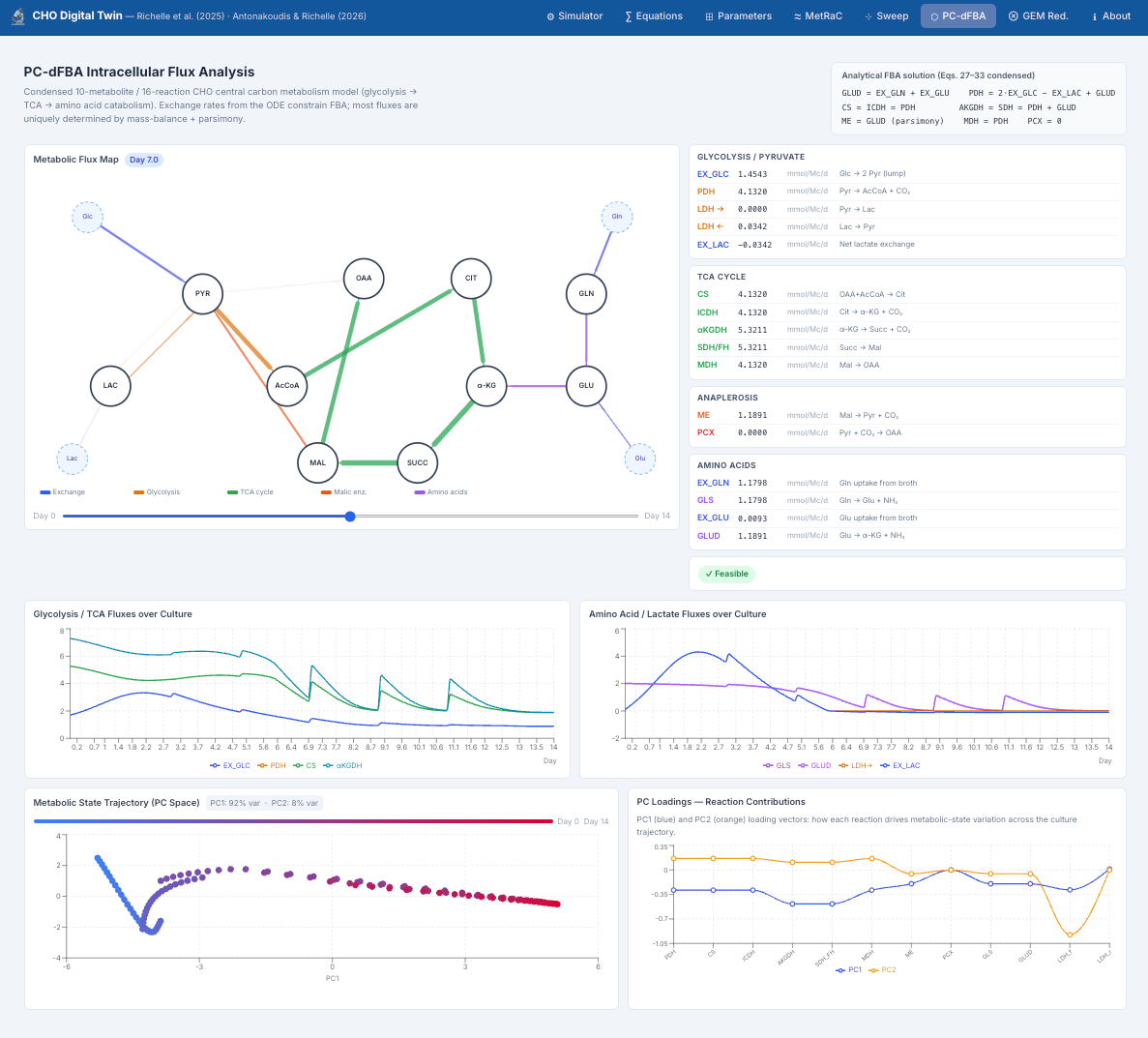
I implemented this analytically for a condensed 10-metabolite, 16-reaction CHO network, so it needs no LP solver in the browser. The flux map renders as a live SVG showing magnitudes and directions across glycolysis, the TCA cycle, amino-acid metabolism and biosynthesis. Click any time point and the whole map updates.

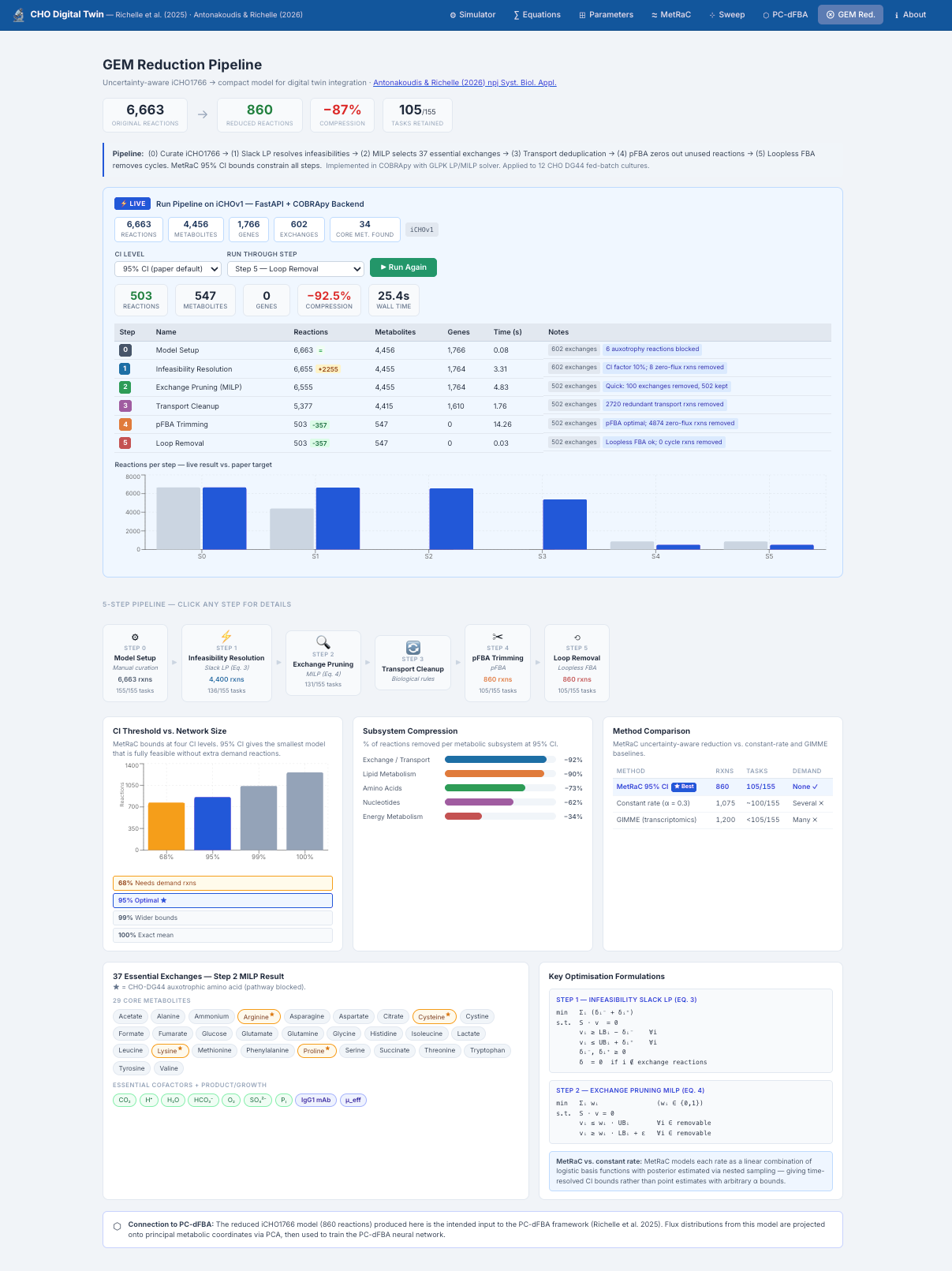
The GEM reduction pipeline: from 6,663 reactions to 503

The condensed network is great for visualisation, but real cells are far more complex. The iCHOv1 genome-scale model (Hefzi et al. 2016) carries 6,663 reactions across 4,456 metabolites — the whole known CHO metabolic network. Running dynamic FBA on all of it would be both computationally brutal and mathematically ill-constrained. The GEM Reduction tab implements the full five-step pipeline from Antonakoudis & Richelle (2026) to compress iCHOv1 into something tractable:

Step 0 — Model curation. Apply the CHO-DG44 auxotrophies: four amino-acid biosynthesis pathways (arginine, cysteine, proline, lysine) are genetically blocked in this line and get disabled. Exchange bounds are set from 57 metabolites measured across all 12 experimental cultures.
Step 1 — Infeasibility resolution (slack LP, Eq. 3). For each time point, check whether the measured exchange bounds are simultaneously achievable. If not, solve an LP that minimises the slack needed to restore feasibility, and add permanent demand reactions for exchanges that stay infeasible across cultures. At 95% CI bounds from MetRaC, zero demand reactions are needed; tighter 68% bounds force ten or more.
Step 2 — Exchange pruning (MILP, Eq. 4). A mixed-integer program finds the smallest subset of exchange reactions that still permits a feasible flux distribution at every time point. Result: 37 essential exchanges — 29 core metabolites, 7 cofactors, the IgG1 product, and growth.
Step 3 — Transport deduplication. Each retained metabolite can usually cross the membrane several ways (passive diffusion, proton-coupled symport, sodium-coupled transport). A biological preference hierarchy keeps the favoured mechanism and drops the redundant routes.
Step 4 — pFBA trimming. Run parsimonious FBA at every time point and remove any reaction that carries zero flux in every parsimonious solution across all time points and objectives. If it never contributes to an observed state, it goes.
Step 5 — Loop removal (loopless FBA). Thermodynamically infeasible cycles can carry flux in standard FBA but not in loopless FBA. Reactions active only inside those impossible cycles are removed.

Result: 6,663 → 503 reactions, a 92.5% compression that still retains 105 of the 155 metabolic tasks defined by Thiele et al. That compact model is what feeds PC-dFBA in the twin. The whole pipeline runs live on a FastAPI + COBRApy backend in roughly 22 seconds, with step results arriving incrementally so you can watch the network shrink in real time.

The seven tabs

🔬 Simulator

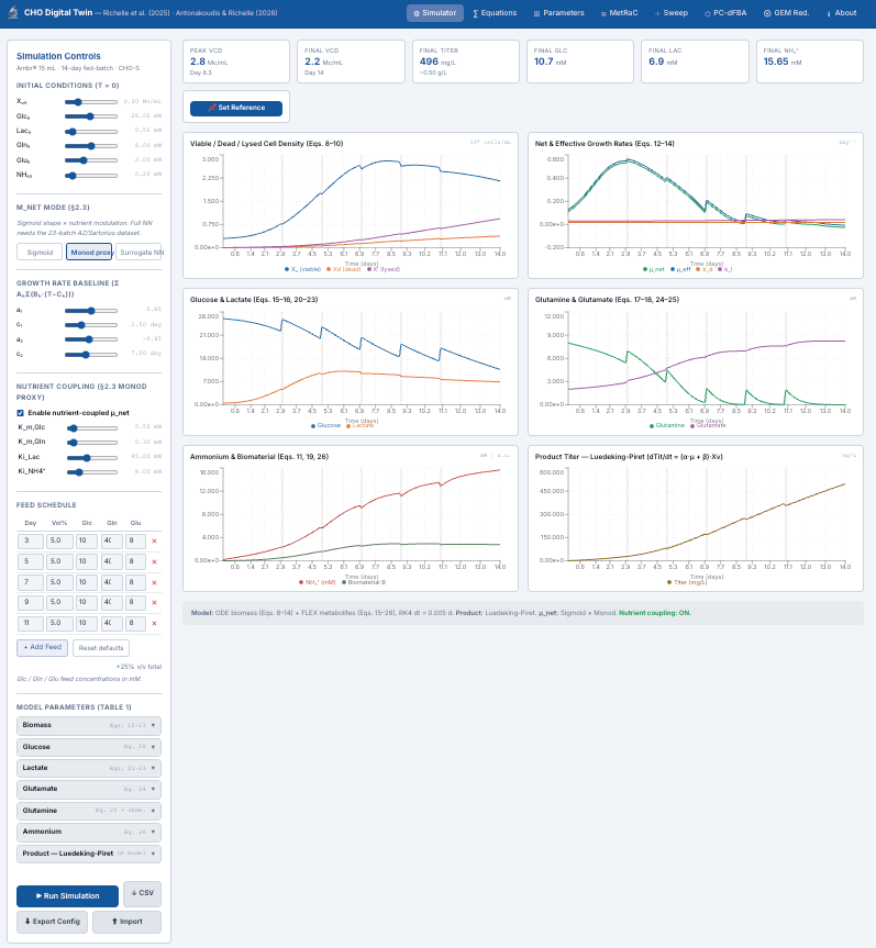
The main one. A 14-day fed-batch runs in under a second via a custom RK45-style ODE integrator written in TypeScript. Six charts update live as you move sliders for initial cell density and metabolites, the logistic growth coefficients (a₁, c₁, a₂, c₂), the nutrient coupling constants (K_Glc, K_Gln, K_I_Lac, K_I_Amm), the feed strategy, and the μ_net mode. KPIs (peak VCD, final titre, final glucose/lactate/ammonium) sit at the top, and a “Set Reference” button locks a run for side-by-side comparison.

Σ Equations

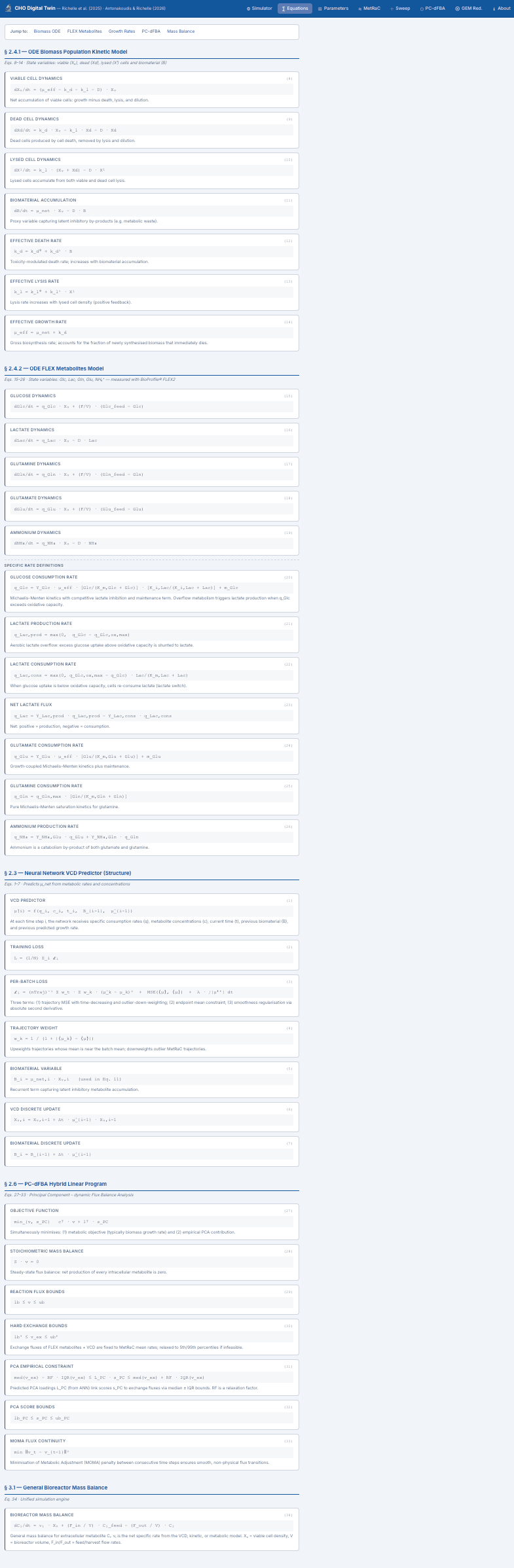
Every equation from the paper (Eqs. 1–26 plus PC-dFBA Eqs. 27–33) rendered cleanly and grouped by subsystem. Hover any one to see its role in the model.

⊞ Parameters

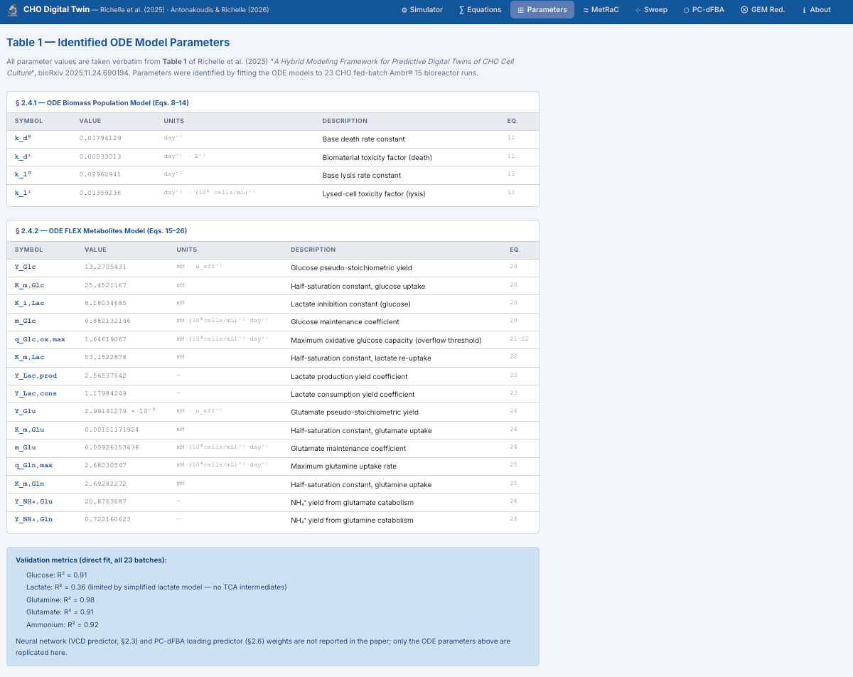
Table 1 as an interactive editor. Change any value and the Simulator uses your set; reset to paper defaults in one click. Each parameter shows its symbol, value, units and the equation it appears in.

≈ MetRaC

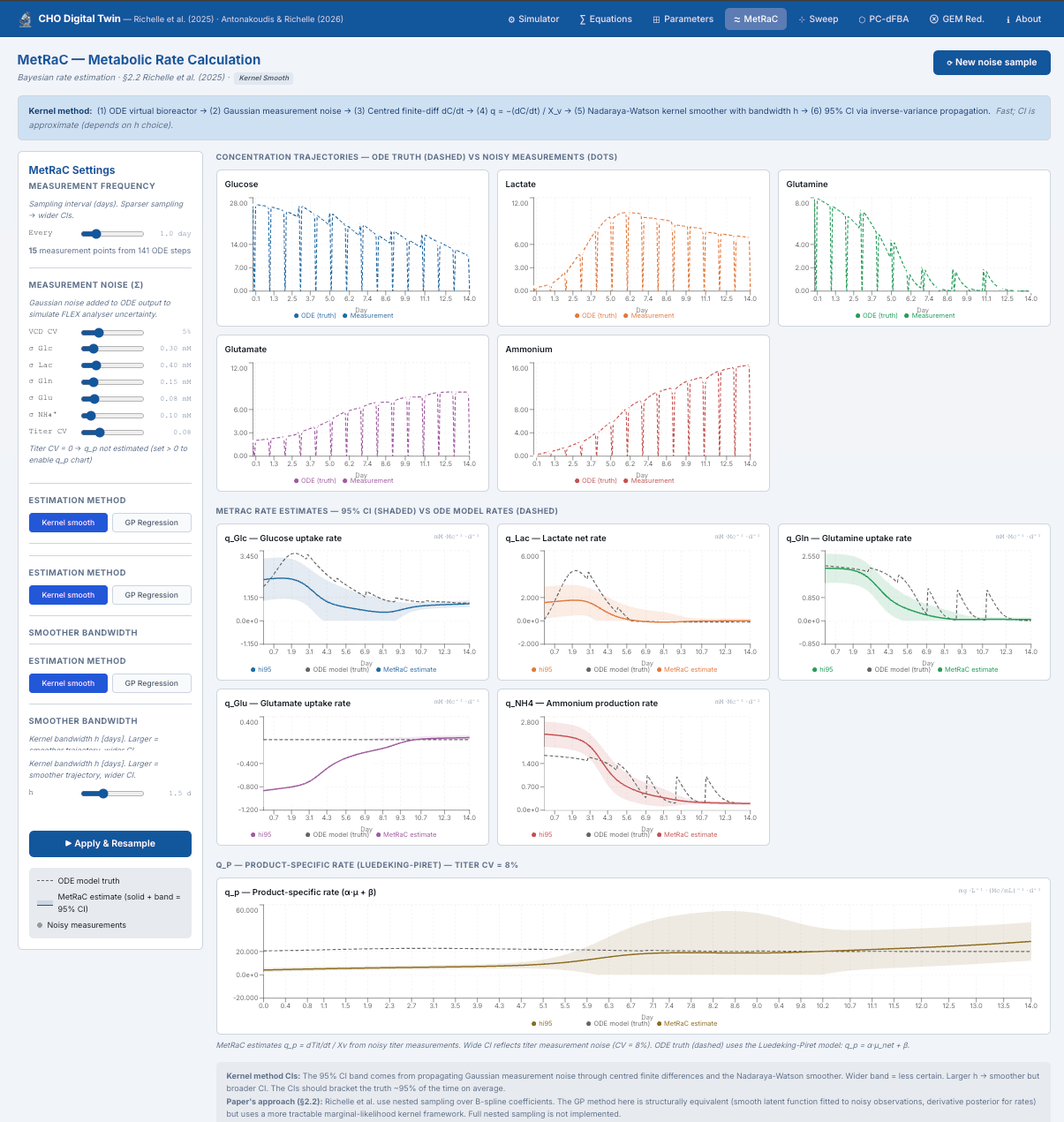
The Metabolic Rate Calculator computes specific exchange rates (q_Glc, q_Lac, q_Gln, q_Glu, q_NH₄, q_mAb) from concentration time series using Gaussian Process regression — the same approach the paper uses to generate the exchange-flux constraints for FBA — with Bayesian 95% credible intervals on each rate. The q_p chart quantifies specific antibody productivity over the run.

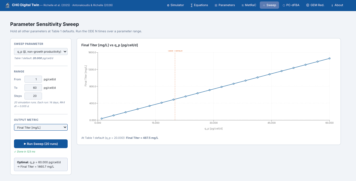
⊕ Sweep

Parameter sensitivity analysis. Pick any parameter, set a range and step, and the app runs the full ODE simulation at every point, plotting final titre, peak VCD and final metabolites against the swept parameter. Good for finding optimal operating points and quantifying how sensitive the process is to each knob.

⬡ PC-dFBA

The intracellular flux view. A live SVG network map (10 metabolite nodes, 16 reaction edges) shows flux magnitudes and directions at any selected time point, with time-series plots of each flux and a PC trajectory plot — the “metabolic fingerprint” of the culture through principal-coordinate space.

⊗ GEM Red.

The live reduction pipeline above. Runs iCHOv1 through all five steps on the FastAPI + COBRApy backend, with incremental step results, a live-versus-paper comparison table, and a waterfall chart of network size at each step.

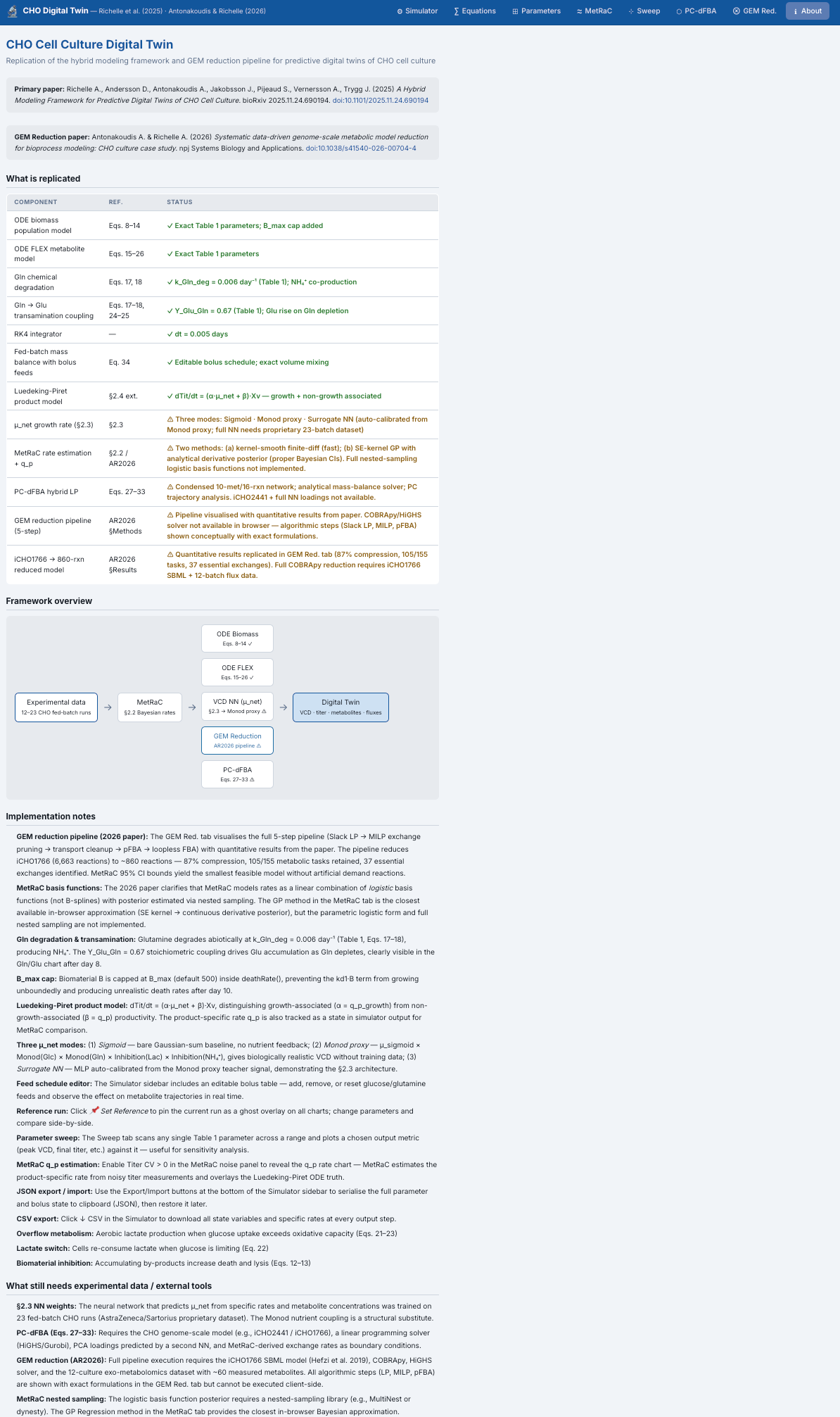
What it’s good for (and what it isn’t)

I want to be honest about the claims here, because bioprocess modelling attracts more hype than it deserves.

Lowering the barrier to entry. Doing this kind of work traditionally means a MATLAB licence, a COBRApy install, a GLPK or Gurobi solver, the original paper’s code, and a few hours of setup before you see anything. Putting it in a browser tab removes all of that. A process-development scientist, a grad student learning metabolic modelling, a reviewer evaluating a manufacturing change — all of them can interact directly with the quantitative framework instead of reading about it.

Making the research reproducible. Reproducibility is a real weak spot in computational biology. Papers give you equations, but the actual implementation — the integrator, the sign conventions, the edge cases — lives in supplementary code that may or may not match the text. This app is a living replication: every equation is numbered to its source, every parameter is from Table 1, and where the app and the paper disagree, the About tab flags it explicitly rather than papering over it.

Compressing development time. The honest use case isn’t “replace the experiment.” It’s “stop exploring blindly.” Suppose your culture peaks on day 8 instead of day 10 and you want to know whether adjusting the day-5 glucose feed would help. The old way is design, order media, run the ambr® for two weeks, analyse, interpret — three to four weeks and tens of thousands of pounds. With the twin, you move a slider, watch the simulation, form a hypothesis, and design a targeted experiment to confirm it. The experiment still happens. It’s just testing a specific, model-derived prediction rather than a hunch.

A template that generalises. The hybrid ODE + FBA + ML architecture isn’t CHO-specific. The same MetRaC uncertainty quantification applies to any exchange-rate measurement, and the same GEM reduction pipeline applies to any organism with a genome-scale model — and there are hundreds: E. coli, yeast, hepatocytes, stem cells. This particular build is CHO-S with an IgG1 product in a 15 mL ambr®, but the methodology and the code are a starting point for a twin of almost any bioprocess.

How it’s built

A TypeScript monorepo managed with pnpm workspaces:

React 19 + Vite 7               ← UI, charts, ODE solver, FBA
     │
     ├─ /gem/*  → Express proxy → FastAPI (Python)
     │                              └─ COBRApy + GLPK
     └─ /api/*  → Express API   ← (future: persistence, auth)

Client-side computation. The ODE simulator, the MetRaC rate calculator, the PC-dFBA analytical solver and the surrogate NN all run entirely in the browser. No server round-trip for any of them — the RK45 integrator runs in TypeScript and finishes a 14-day simulation in under 50 ms.

Server-side COBRApy. The GEM reduction needs an LP/MILP solver (GLPK) and COBRApy, so it runs on a FastAPI backend with a job-queue pattern: POST /gem/run-pipeline returns a job ID immediately, and the browser polls GET /gem/job/{job_id} every 1.5 seconds while the ~22-second pipeline streams its step results back.

A few design decisions that earned their keep:

The iCHOv1 model (5.6 MB JSON) is loaded once at startup and cached as a pickle — roughly 0.12 s to copy from cache versus ~2.5 s to reparse the JSON. Each run gets a fresh copy.
The Express proxy runs no body-parsing middleware before the proxy block. This one cost me time: express.json() consumes the request stream, which silently breaks http-proxy-middleware’s ability to forward POST bodies.
ODE state is immutable between steps; the integrator returns the full trajectory array, so rendering any time range is trivial and never re-runs the simulation.

The papers behind it

Richelle et al. (2025). Integrating mechanistic and machine learning models for predictive digital twins of CHO cell culture. bioRxiv 2025.11.24.690194. This is the source for the hybrid ODE + PC-dFBA + surrogate NN framework behind the Simulator, Equations, Parameters, MetRaC, Sweep and PC-dFBA tabs — the 26 kinetic equations, the three μ_net variants, the MetRaC Bayesian rate estimation, and the PC projection.

Antonakoudis & Richelle (2026). Uncertainty-aware genome-scale model reduction for dynamic flux balance analysis of CHO cell culture. npj Systems Biology and Applications. This is the source for the five-step reduction in the GEM Red. tab — how MetRaC credible-interval bounds constrain the MILP exchange-pruning step, why 95% CI is the sweet spot (smallest model, no demand reactions), and how their resulting 860-reaction network reaches 87% compression while keeping 105/155 tasks. The live app pushes that to 92.5% (503 reactions) using a quick-mode MILP solve.

Hefzi et al. (2016). A Consensus Genome-scale Reconstruction of Chinese Hamster Ovary Cell Metabolism. Cell Systems 3(5):434–443. The iCHOv1 model that feeds the reduction pipeline.

What’s next

The app today is a faithful replication of two frameworks. Where I want to take it:

Multi-culture parameter estimation — fit the 40+ parameters to a user-uploaded concentration dataset via Bayesian inference (nested sampling or MCMC), replicating the full calibration workflow.
Scale-up prediction — extend to 200 L and 2,000 L with mixing-time and oxygen-transfer corrections.
Process optimisation — wrap the twin in an optimisation loop to find feed strategies that maximise titre subject to quality constraints.
Real-time monitoring — connect to live bioreactor streams for continuous state estimation via moving-horizon estimation.

Getting it

The full source is on GitHub: github.com/lynchaos/cho-digital-twin. Clone it and you can run the whole thing locally — the front end and the COBRApy backend.

There’s no public hosted instance up at the moment. I’m planning to put one online soon, and when it is, this is what I’d point you at first: open the GEM Red. tab and hit Run Pipeline to watch 6,663 reactions collapse to 503 in real time, then drop the CI selector to a tighter bound and see how that forces extra demand reactions — the exact trade-off that motivates the whole MetRaC framework. Then head to the Simulator, push the initial glutamine to 12 mM, and watch ammonium climb to toxic levels by day 4. Switch to Surrogate NN mode and notice it captures the same growth dynamics with a completely different mathematical representation underneath. That’s the hybrid model doing its job.

I’ll update this post with the live URL the moment it’s up.

Built with React 19, TypeScript, Recharts, FastAPI, COBRApy, and a lot of stoichiometry.