Beyond the 2D Bounding Box: Why Bioimage Deep Learning Is a Completely Different Beast and How BiaPy Tames It

https://github.com/lynchaos/biapy-hub

https://lynchaos-biapy-hub-app-hlcmfj.streamlit.app/

Thank you for reading this post, don't forget to subscribe!

If you have spent your machine learning career optimizing ResNets or YOLO on ImageNet and COCO, here is an inconvenient truth: standard computer vision has spoiled you.

In standard computer vision, a batch is usually an RGB triplet $(B, 3, H, W)$ where $H, W \le 1024$ . The pixels are isotropic, the spatial coordinates are Euclidean, the lighting is roughly Lambertian, and if your GPU runs out of VRAM, you just drop the batch size from 64 to 32 and call it a day.

Then you step into a bioimaging core facility.

Suddenly, you are handed a 5D tensor $(T, C, Z, Y, X)$ representing a multi-terabyte volumetric light-sheet stack or a whole-slide histopathology gigapixel image. Your axial resolution ( $Z$ ) is 4x worse than your lateral resolution ( $XY$ ) due to optical Point Spread Function (PSF) elongation. Your raw data is corrupted by Poisson-Gaussian mixed shot noise. Your cells are packed like sardines in a 3D spheroid, touching each other with zero background margin. And to top it off, loading a single time-point uncompressed into memory would cause your workstation’s kernel to invoke the OOM-killer before PyTorch even initializes its CUDA context.

This is where standard computer vision tooling breaks down, and where frameworks engineered specifically for bioimage spatial intelligence, most notably BiaPy become indispensable. Here is an under-the-hood look at the mathematics, optical physics, and distributed systems engineering required to run deep learning on massive bioimage datasets without losing your sanity.

—

1. The Geometry of the Problem: Anisotropy and the 3D PSF

In microscopy, we don’t capture ideal mathematical points; we capture the convolution of the specimen’s fluorophore distribution $\rho(\mathbf{r})$ with the microscope’s Point Spread Function (PSF) $h(\mathbf{r})$ :

$I(\mathbf{r}) = (\rho * h)(\mathbf{r}) + \eta_{\text{Poisson}}(\mathbf{r}) + \eta_{\text{Gauss}}(\mathbf{r})$

The lateral resolution is bounded by the classical Abbe diffraction limit:

$d_{xy} = \frac{\lambda}{2 \cdot \text{NA}}$

While the axial resolution along the optical axis ( $Z$ ) degrades quadratically with the Numerical Aperture:

$d_{z} = \frac{2 \cdot \lambda \cdot n}{\text{NA}^2}$

$\text{Aspect Ratio} = \frac{d_z}{d_{xy}} = \frac{4 \cdot n}{\text{NA}} \approx 3.5 \text{ to } 4.5$

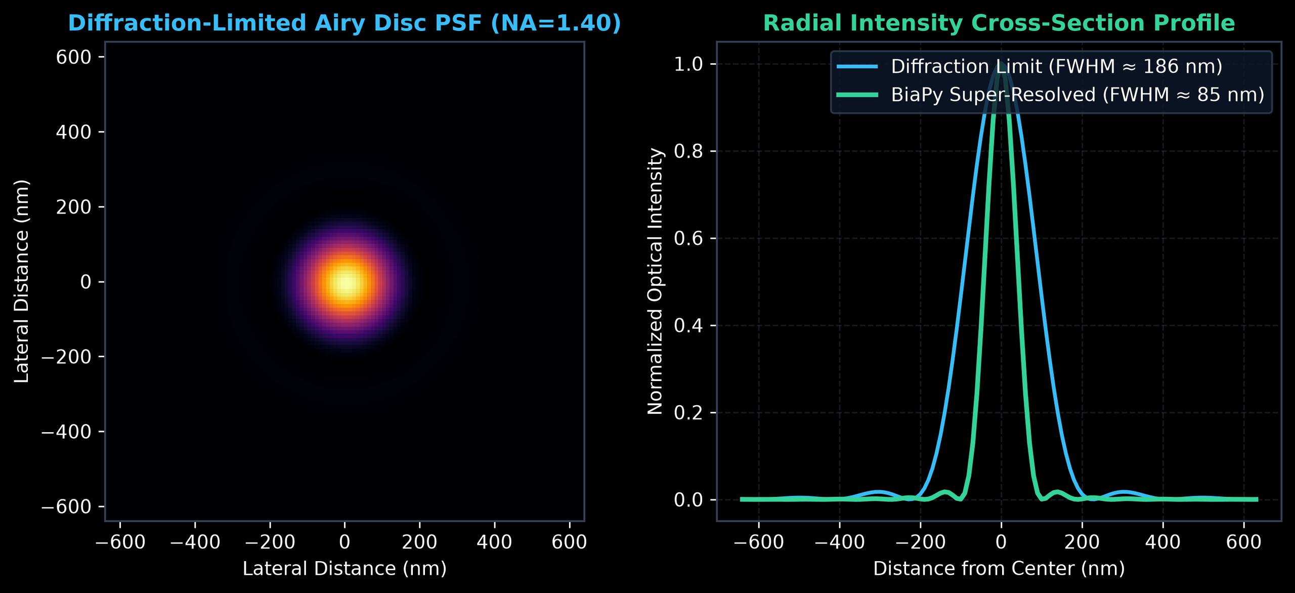
If you feed this volume into a standard 3D CNN with symmetric $3 \times 3 \times 3$ kernels, the network treats 1 pixel in $Z$ as physically equivalent to 1 pixel in $XY$ . The result? Severe axial blur, cross-slice topological disconnects, and over-segmentation.

BiaPy handles this natively through anisotropic pooling architectures (e.g., `Z_DOWN: [1, 2, 2, 2]`), where early convolutional downsampling occurs strictly across $XY$ while keeping $Z$ stride at 1 until the receptive field matches the true physical aspect ratio $\Delta z / \Delta xy$ .

—

2. The Multi-Terabyte Dilemma: Artifact-Free Overlapping Chunking

When an image volume is $10{,}000 \times 10{,}000 \times 500$ voxels (approx. 93 GB uncompressed uint16), you cannot perform a single forward pass. You must chunk the tensor into patches $\Omega_i$ , run inference per tile, and stitch them back into the global space $\Omega$ .

The Boundary Artifact Trap

The naive approach—tiling with zero overlap—creates boundary seamlines along the borders because convolutions near tile edges suffer from zero-padding boundary bias and missing receptive fields.

To eliminate tile boundaries, BiaPy employs an overlap cushion with multi-dimensional Gaussian/Cosine apodization blending windows:

$I_{\text{stitched}}(\mathbf{x}) = \frac{\sum_{i} \mathcal{W}_i(\mathbf{x}) \cdot \hat{y}_i(\mathbf{x})}{\sum_{i} \mathcal{W}_i(\mathbf{x})}$

where the spatial weighting function $\mathcal{W}_i(\mathbf{x})$ smoothly attenuates near tile edges:

$\mathcal{W}_i(x, y) = \sin^2\left(\frac{\pi x}{L_x}\right) \cdot \sin^2\left(\frac{\pi y}{L_y}\right)$

This mathematical weighting guarantees that predictions originating from the high-confidence center of patch $A$ smoothly dominate the low-confidence boundaries of patch $B$ , producing zero visible seamlines across gigapixel scans.

—

3. Disentangling 3D Crowds: From Binary Masks to Watershed Topologies

In biological tissue, cells aren’t floating in clean isolation. In a tumor organoid or an embryonic blastocyst, cell membranes touch continuously.

A standard semantic segmentation head predicting binary foreground $\hat{Y} \in \{0, 1\}$ merges the entire cluster into one massive, unsegmented clump.

To solve this without throwing massive computational overhead at 3D anchor-based proposal networks (like 3D Mask R-CNN), BiaPy implements Multi-Task Boundary-Central (BC) and Boundary-Central-Distance (BCD) vector representations:

1. Channel 1 (B): Binary cell interior.

2. Channel 2 (C): Cell-cell contact boundaries / contours.

3. Channel 3 (D): Euclidean Distance Transform map $\mathcal{D}(\mathbf{x}) = \min_{\mathbf{y} \in \partial \Omega} \|\mathbf{x} - \mathbf{y}\|_2$ , parameterized as topological seeds for marker-controlled watershed transform.

By extracting topological seed markers at local maxima:

$S_k = \text{LocalMaxima}\left(\mathcal{D}(\mathbf{x}) \cdot \mathbb{I}_{\{C(\mathbf{x}) < \tau_c\}}\right)$

and running topological flooding on the inverted distance gradient landscape $\nabla \mathcal{D}$ , touching cells are separated with exact boundary preservation in full 3D space.

—

4. Virtual Staining: Image-to-Image Optical Phase Inversion

One of the most exciting capabilities in modern bioimaging is Virtual Staining using deep networks (e.g., 2D/3D UNETR, RCAN) to predict synthetic multi-channel fluorescence directly from label-free transmitted light (brightfield / phase-contrast).

Why does this matter? Fluorescence imaging requires phototoxic lasers and chemical fluorophores that kill live cells over extended time-lapse experiments. Phase-contrast microscopy is non-destructive, but human eyes cannot resolve specific organelle protein structures from phase shifts alone.

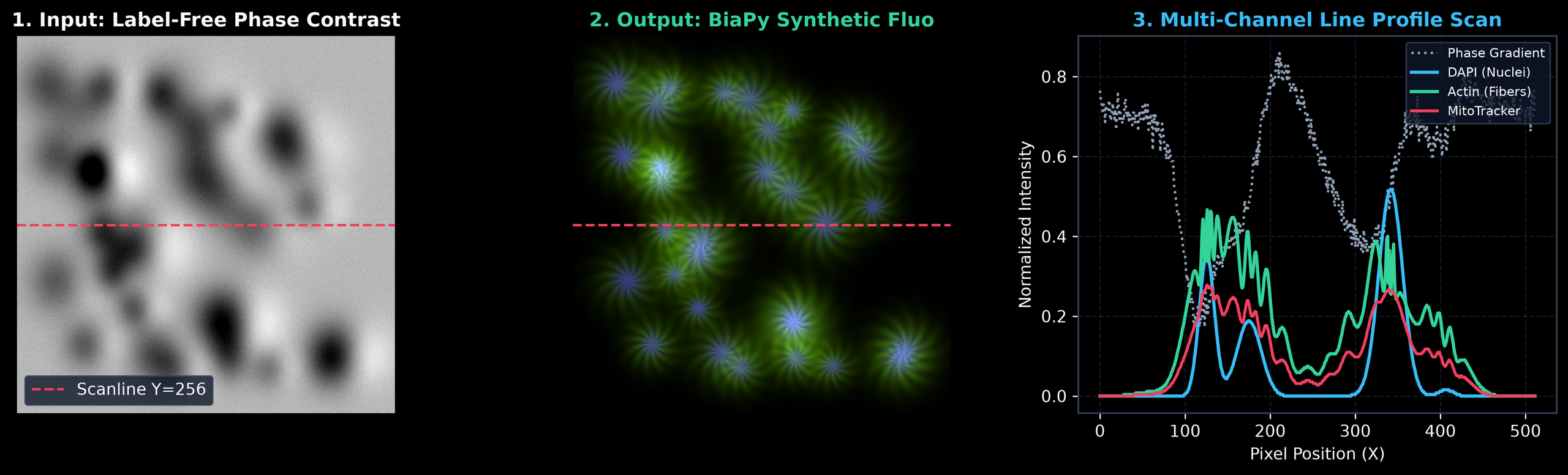
The network learns the non-linear inverse mapping from optical phase gradients to molecular density:

$\mathcal{L}_{\text{staining}} = \alpha \|\hat{Y} - Y\|_1 + (1 - \alpha) \left(1 - \text{SSIM}(\hat{Y}, Y)\right) + \beta \mathcal{L}_{\text{gradient}}$

The structural similarity ( $\text{SSIM}$ ) term ensures that high-frequency cellular actin filaments are preserved rather than averaged out by standard $L_2$ regression blur.

—

5. Quantitative Spatial Point Processes: Ripley’s Besag L-Function

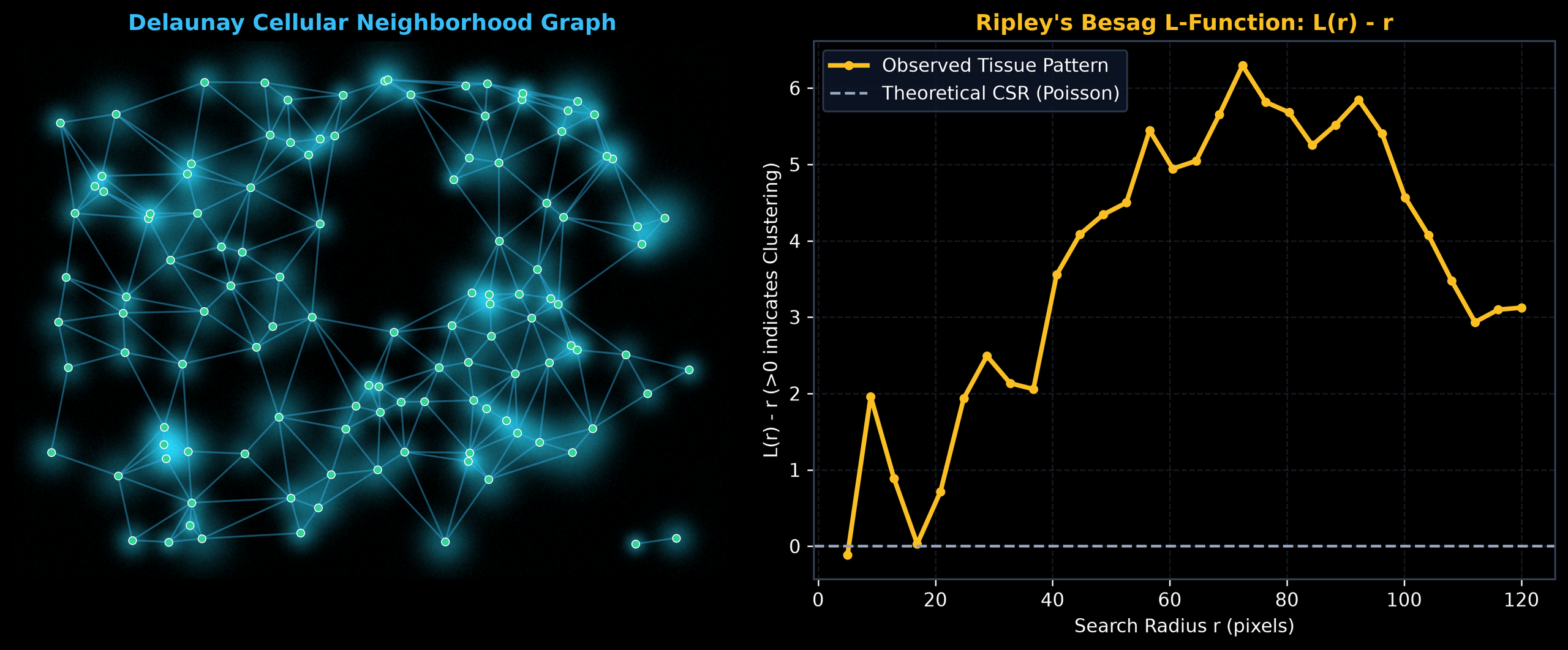
Once BiaPy detects 50,000 cells across a whole-slide tissue section, the job isn’t done. Biologists don’t just want counts; they want spatial architecture. Are immune lymphocytes infiltrating the tumor core, or are they excluded at the stroma?

To mathematically evaluate spatial patterns beyond simple density histograms, we use Ripley’s $\mathbf{K-}$ function and Besag’s $\mathbf{L-}$ transformation:

$\mathbf{L(r) - r \gt 0}$ : Statistically significant spatial aggregation / clustering (e.g. tumor nests, immunological hubs).

$\mathbf{L(r) - r = 0}$ : Complete Spatial Randomness (Poisson point process).

$\mathbf{L(r) - r \lt 0}$ : Regular spacing / contact inhibition.

* $\mathbf{L(r) - r > 0}$ : Statistically significant spatial aggregation / clustering (e.g. tumor nests, immunological hubs).

* $\mathbf{L(r) - r = 0}$ : Complete Spatial Randomness (Poisson point process).

* $\mathbf{L(r) - r < 0}$ : Regular spacing / contact inhibition.

—

6. The Engineering Bridge: Zero-Code Declarative YAML to Production

The dirty secret of AI in biology is the “deployment chasm.” Brilliant models written in custom PyTorch scripts die in Jupyter notebooks because bench biologists work in Fiji / ImageJ and digital pathologists work in QuPath.

BiaPy bridges this divide by making every single workflow completely declarative through a single YAML specification:

SYSTEM:

  NUM_WORKERS: 8

PROBLEM:

  TYPE: INSTANCE_SEG

  NDIM: 3D

DATA:

  PATCH_SIZE: (32, 128, 128, 1)

  TRAIN:

    PATH: /data/organoids_3d/train

  TEST:

    PADDING: (4, 16, 16)

    OVERLAP: (8, 32, 32)

MODEL:

  ARCHITECTURE: RESUNET_3D

  FEATURE_MAPS: [28, 36, 48, 64]

  Z_DOWN: [1, 2, 2, 2]

POST_PROCESSING:

  WATERSHED: true

  WATERSHED_SEEDS_TH: 0.85

This single declarative file configures data loading, GPU memory allocation, mixed-precision (AMP), distributed data parallel (DDP) training across multi-GPU nodes, evaluation metrics (Jaccard, Hausdorff Distance, F1), and automated export into the open BioImage Model Zoo specification (`model.yaml` RDF).

—

The Interactive Hub: Putting Theory into Practice

https://lynchaos-biapy-hub-app-hlcmfj.streamlit.app

To demonstrate these principles live, we built the BiaPy Interactive Hub. A multi-module scientific workstation that couples these deep learning pipelines with interactive visualization tools:

* Real-time 3D Mesh Inspection: Marching Cubes isosurface extraction rendered via Three.js WebGL with $360^\circ$ OrbitControls and live clipping planes.

* Calibrated Cross-Section Line Scans: Pixel-accurate lateral intensity profiles comparing phase contrast gradients against multi-channel synthetic signals.

* Spatial Delaunay Topology & Point Processes: Live nearest-neighbor distance distributions and Besag $L(r)-r$ clustering evaluations.

* Interoperability Bridges: One-click generation of QuPath Groovy scripts, Fiji macros, and BioImage.io RDF packages.

Bioimage analysis is moving past ad-hoc manual thresholding into an era of reproducible, multi-dimensional deep spatial intelligence. If you are handling large-scale biological datasets, it’s time to build pipelines that respect both the machine learning and the underlying optical physics.

Leave a Reply Cancel reply