
Look, I’ll be honest. For years I ran bioreactors the way most of us do: set your temperature, set your pH, watch the DO trace, take a sample every few hours, and hope for the best. You tweak the feed rate because “it feels right.” You crank up the stirrer because the DO is dropping. You tell yourself you understand the process. You don’t. Not really.
Thank you for reading this post, don't forget to subscribe!I’m a bioreactor engineer. I spent years designing and running fermentations the conventional way — Monod kinetics on paper, PID loops on everything, and a lot of gut feeling in between. Then I discovered what machine learning and model predictive control can actually do for upstream bioprocessing, and I haven’t looked back.
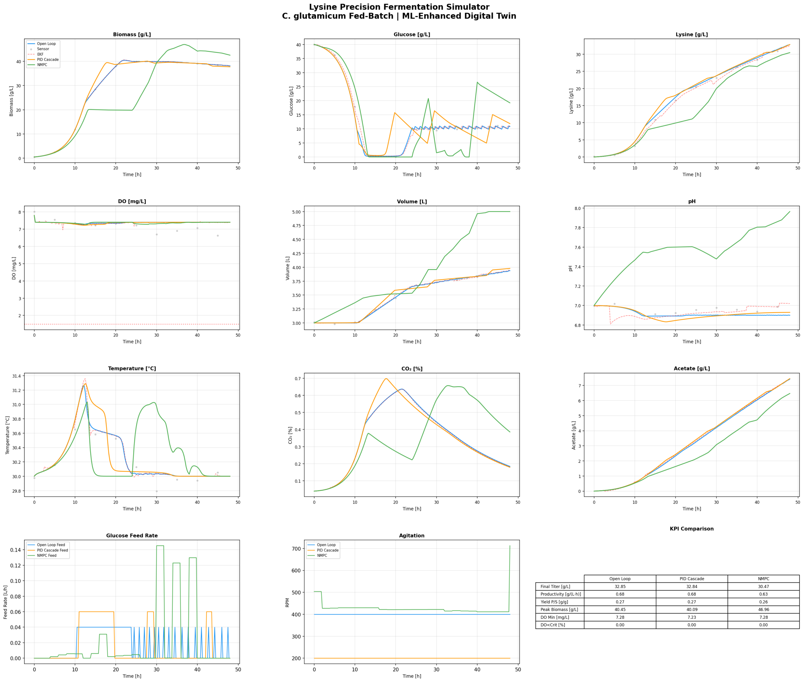
This post is about lysine production with Corynebacterium glutamicum — one of the workhorses of industrial amino acid fermentation — and what happens when you stop treating your bioreactor like a black box and start treating it like a system you can actually predict and control in real time.
The Problem With How We Usually Do Things
Traditional lysine fermentation is a fed-batch process. You inoculate, you grow your biomass, you feed glucose, and C. glutamicum does its thing — shunting carbon through the aspartate pathway to make L-lysine. The kinetics are well-characterised. Monod growth with substrate inhibition (Andrews kinetics), Luedeking-Piret production, product inhibition, overflow metabolism producing acetate when you overfeed. Nothing exotic.
The problem isn’t the biology. The biology is fine. The problem is how we control it.
A typical setup: PID on DO controlling agitation and airflow, PID on pH controlling base addition, and some threshold-based feeding strategy — “when glucose drops below 10 g/L, turn the pump on.” Maybe you’ve got a cascade. Maybe you’ve even tuned your PIDs properly (most people haven’t, and that’s okay, it’s painful work).
But here’s the thing — PID doesn’t know where your process is going. It only knows where it is right now, and even that information is noisy, delayed, and sometimes drifting. Your DO probe drifts. Your glucose measurement is at-line with a 30-minute delay. Your HPLC result for lysine comes back hours later. You’re flying half-blind and reacting to the past.
What Changes When You Add ML
The shift isn’t about replacing biology with algorithms. It’s about giving yourself better eyes and a better brain for the process.
Here’s what I’ve been building and what I think actually matters:
State Estimation: Know Where You Actually Are
Extended Kalman Filters and Unscented Kalman Filters are game-changers for bioprocesses. You have a mechanistic model — your ODEs, your Monod kinetics, your mass balances — and you have noisy sensor data. The Kalman filter fuses them. It gives you a best estimate of your actual state, including variables you can’t measure directly.
Your DO probe is drifting? The EKF compensates. Your glucose reading is delayed by 30 minutes? The UKF propagates the model forward and corrects when the measurement arrives. You want to know your real-time specific growth rate without waiting for an OD sample? The filter estimates it.
I use the UKF more than the EKF these days. Bioprocess kinetics are highly nonlinear — the sigma-point approach handles that better than linearising around your current state with a Jacobian. Yes, it’s more computationally expensive (you’re propagating 21 sigma points through your ODE system at every time step), but we’re not doing high-frequency trading here. We have time.
Soft Sensors: Measure What You Can’t Measure
Gaussian Process regression soft sensors are probably the most immediately useful ML tool for fermentation. The concept is simple: you train a GP to predict a hard-to-measure variable (lysine concentration, viable cell density) from easy-to-measure ones (DO, pH, temperature, off-gas CO₂, time).
The beauty of GPs is the uncertainty quantification. You don’t just get a prediction — you get a confidence interval. When the GP tells you “lysine is approximately 35 g/L ± 2.1 g/L,” that ± 2.1 matters. It tells you how much to trust the prediction. If the uncertainty suddenly spikes, something unusual is happening — maybe the process has drifted outside the training distribution, maybe a sensor is failing.
I use a Matérn 5/2 kernel plus RBF plus white noise, with online sliding-window retraining. It works well for the smooth, continuous dynamics you see in fed-batch fermentation.
Model Predictive Control: Know Where You’re Going
This is where it gets really interesting. Nonlinear MPC doesn’t just react to the current state — it predicts the future trajectory of your process over a horizon (say, 5 hours ahead), and optimises your control actions to maximise an objective function.
For lysine production, my objective is roughly: maximise lysine productivity, keep DO above the critical threshold (about 20% saturation — you don’t want oxygen limitation during production phase), don’t waste glucose, and don’t make jerky control moves.
The NMPC solves this optimisation problem at every control interval, taking into account the full nonlinear model. It knows that if you increase the feed rate now, glucose will rise, growth will accelerate, oxygen demand will spike, and DO will drop — so it pre-emptively adjusts agitation and aeration before the DO crash happens. A PID can never do that. It has to wait for the error to appear.
The computational cost is real. You’re solving a constrained nonlinear optimisation every few minutes. That’s why I use a neural network surrogate model — an MLP trained on the mechanistic model’s input-output space — to speed up the trajectory predictions inside the MPC loop. The surrogate is 100x faster than solving the ODEs, and accurate enough for control purposes.
Anomaly Detection: Know When Something Is Wrong
Contamination, sensor faults, unexpected metabolic shifts — these things happen, and they don’t always announce themselves obviously. By the time you see a pH crash or a sudden DO spike, you’ve already lost hours.
I run a multi-model anomaly detection system in parallel with the process: Isolation Forest for multivariate outlier detection, an autoencoder that flags high reconstruction error, Hotelling’s T² for statistical process control, and simple rate-of-change monitoring. Ensemble vote: if two or more methods flag an anomaly, it’s worth investigating.
It’s not perfect. You’ll get false positives, especially during phase transitions (lag to exponential, exponential to stationary). But I’d rather investigate a false alarm than miss a real contamination event at hour 30 of a 48-hour batch.
The Hybrid Approach: Physics + Data
Pure ML models are dangerous in bioprocessing. Train a random forest on 50 batches and it’ll interpolate beautifully within that operating space. Push it outside — different strain, different media, slightly different temperature — and it’ll give you confident nonsense.
That’s why I use physics-informed hybrid models. The mechanistic model (your ODEs, your mass balances, your thermodynamics) provides the structure. An ML component learns the residual — the systematic mismatch between what your first-principles model predicts and what actually happens. The ML corrects for things like unmodelled metabolic regulation, media batch variability, or imprecise kinetic parameters.
The key constraint: the hybrid model still has to obey physics. Mass balances must close. Substrate consumption can’t be positive during active growth. Production rate can’t be negative. You enforce these as hard constraints on the ML correction. This gives you a model that’s both accurate within the training domain and physically sensible outside it.
What I’ve Actually Seen
Running NMPC against PID on the same process, same initial conditions, same 48-hour fed-batch: NMPC consistently delivers higher lysine titres and better productivity. Not because it’s magic — because it makes better feeding decisions. It feeds less glucose during lag phase (less overflow metabolism, less acetate), ramps up feeding in sync with oxygen transfer capacity during exponential phase, and manages the transition to production phase more smoothly.
The DO trace under NMPC is boring. That’s good. Boring means controlled. Under PID, you see the classic oscillations — overshoot, undershoot, the controller chasing the setpoint. Under NMPC, the DO stays in a comfortable range because the controller anticipated the oxygen demand before it arrived.
Being Honest About The Limitations
None of this is plug-and-play. Training the ML components requires good data, which means you need a decent mechanistic model to start with (or a lot of historical batch data). The NMPC optimisation can be slow — you need a surrogate model or a fast computer. The Kalman filters need sensible noise covariance matrices, which means you need to characterise your sensors.
And the biggest limitation: your mechanistic model is always wrong. It’s a simplification. C. glutamicum metabolism is vastly more complex than a Monod equation and a Luedeking-Piret model. The model doesn’t know about phage infections, or subtle media lot-to-lot variability, or that one probe that’s been slightly off-cal for two days. The ML components help patch over some of this, but they’re not omniscient.
The point isn’t perfection. The point is doing better than “set it and forget it.” And on that front, the ML-enhanced approach delivers. Consistently.
Where This Is Going
The endgame is fully autonomous fermentation. Not “AI replaces the engineer” — that’s nonsense. More like “AI handles the minute-to-minute control decisions so the engineer can focus on process development, troubleshooting, and strategy.”
Reinforcement learning is interesting here. Train an agent through thousands of simulated batches to learn optimal feeding and control strategies. It’s early days — tabular Q-learning on a discretised state space is crude compared to what you’d want for production — but the trajectory is clear.
Bayesian optimisation for process parameters is already practical. Instead of running 50 DoE batches to find optimal temperature, pH, and feed strategy, you run 8 initial experiments, build a GP surrogate, and let Expected Improvement guide you to the optimum in 15-20 batches. That’s real time and money saved.
Digital twins — real-time mechanistic models running in parallel with your physical bioreactor, continuously updated by sensor data through Kalman filtering — are the foundation for all of this. The twin predicts, the sensors correct, the controller optimises, the anomaly detector watches. It’s a system, not a single algorithm.
Final Thought
I’m not writing this as someone who was always into ML. I came from the conventional side. I designed bioreactors with spreadsheets and experience and rule-of-thumb feeding strategies. The transition to coding in Python, building ODE models, training GPs and neural networks — it was steep. But the results speak for themselves.
If you’re a bioprocess engineer who’s curious about this stuff but hasn’t made the jump yet: start with a Kalman filter on one of your existing processes. Just the state estimation. See what it tells you about your process that your sensors alone can’t. That’s the moment it clicks.
The biology hasn’t changed. C. glutamicum is still doing the same metabolic work it always did. What’s changed is how well we can see it, predict it, and guide it. And that makes all the difference.
The Bioreactor Production Details!
https://kemal.yaylali.uk/running-a-5-litre-lysine-fermentation-from-scratch-everything-nobody-tells-you/