Simulating the Corpus Clock: A Hybrid Dynamical Systems Model of Taylor’s Chronophage

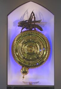
The Corpus Clock sits at the corner of Corpus Christi College, Cambridge. Unveiled in 2008 by Stephen Hawking, it was designed by inventor John C. Taylor as a meditation on time’s relentless consumption of life. A giant golden insectoid sculpture — the Chronophage (from the Greek chronos, time, and ephagon, I ate) — crouches atop the clock face, its jaw mechanically opening and closing as it devours the passing seconds.

What fascinated me about this clock is that it’s deliberately inaccurate. Taylor built in numerous mechanical “tricks” — stalls, surges, hesitations — that cause the displayed time to wander unpredictably. It’s “entirely accurate only once every five minutes.” The inscription below reads: mundus transit et concupiscentia eius — “the world passeth away, and the lust thereof.”

I wanted to see if I could reproduce this behaviour in code. What came out is a hybrid dynamical system: a continuous nonlinear ODE for the pendulum, impulsive events for the escapement, a stochastic finite-state machine for the tricks, and periodic discrete corrections for the phase lock. If you’ve ever worked with fed-batch bioreactor models — impulsive feeding, stochastic disturbances, periodic recalibration — the structure will feel very familiar.

A note on accuracy. The internal mechanism of the Corpus Clock is proprietary. Parameters like the pendulum length, tooth count, and the exact trick mechanisms aren’t publicly documented. I’ve used physically plausible values chosen to reproduce the qualitative behaviour reported in public sources, and I flag every assumption below.

The Pendulum and Escapement

At the heart of every mechanical clock is an oscillator. The Corpus Clock uses a physical pendulum — I assume an effective length L ≈ 0.994 m, tuned for a natural period of about 2 seconds (one full swing per second in each direction).

The equation of motion is the classic nonlinear damped pendulum:θ̈ + 2ζω₀θ̇ + ω₀² sin(θ) = Q(t) / I

where:

• θ — pendulum angle from vertical (state variable)
• ω₀ = √(g/L) — natural angular frequency ≈ π rad/s (assumed L)
• ζ = 0.0015 — damping ratio (typical low-friction pendulum; assumed)
• I = 1.0 — effective moment of inertia (normalised/scaled)
• Q(t) — total applied torque = Q_esc + Q_reg

I kept the full sin(θ) nonlinearity rather than linearising to θ. At the operating amplitude θ* ≈ 0.12 rad (≈ 7°), the difference is small, but the nonlinear form preserves amplitude-dependent frequency shifts that become visible during the tricks. The ODE is integrated with a classical fourth-order Runge–Kutta scheme at a fixed step of Δt = 5 ms — roughly 400 steps per pendulum period.

The grasshopper escapement

A pendulum in air loses energy every cycle. The escapement’s job is to inject just enough energy to replace what dissipation removes, keeping the oscillation at a stable amplitude.

Taylor’s grasshopper escapement is a variant of the classical Harrison design. In the real mechanism, the pallets push the pendulum continuously throughout its swing — they never disengage. This is fundamentally different from a deadbeat escapement.

I simplified this to an instantaneous velocity impulse at each pendulum zero-crossing:Δθ̇ₖ = (A / I) · sign(θ̇ₖ)

and advance the escape-wheel angle by half a tooth:φ ← φ + π / N_teeth

Two zero-crossings make one full pendulum period, advancing the wheel by one tooth. With N_teeth = 60 (assumed), one full rotation corresponds to 60 seconds — exactly one minute. This impulse approximation is standard in horological modelling. It preserves the correct energy-balance behaviour but doesn’t capture the continuous pallet–pendulum interaction of the real grasshopper.

Energy balance

The impulse amplitude A is tuned so that energy injection balances dissipation at the target amplitude θ*. In the small-angle, linear-damping regime:E_diss/cycle ≈ 2π · ζ · I · ω₀ · θ*²E_inj/cycle ≈ 2 · A · θ* · ω₀

Setting these equal:A = π · ζ · I · θ* ≈ 5.65 × 10⁻⁴ N·m·s

for ζ = 1.5 × 10⁻³ and θ* = 0.12 rad. This self-consistency ensures the pendulum settles onto a stable limit cycle. The simulation checks for zero-crossings at each time step, with a debounce guard of at least 0.3 s since the last impulse to prevent double-triggering — mirroring the mechanical detent in a real escapement.

Tricks, Phase-Lock, and Display

This is where the Corpus Clock departs from every other clock in the world. Taylor deliberately introduced mechanical “tricks” that make the displayed time wander. The pendulum “speeds up, slows down, and sometimes stops.”

In reality, these tricks are generated by purely mechanical means — countwheels with “semi-random spacing,” cams, and spring-loaded detents. No computer, no electronics. The clock is “entirely mechanically controlled, without any computer programming.” The roughly fifty distinct behaviours are deterministic sequences that merely appear random to the observer.

I modelled this as a continuous-time Markov chain with four states — which produces statistically similar output even though the underlying mechanism is fundamentally different from the real thing:

• NORMAL — no extra torque; the clock ticks normally.
• STALL — heavy damping (ζ_eff = ζ + 0.25); the pendulum amplitude decays rapidly toward zero. The escape wheel stalls — displayed time freezes. Transition rate: 0.006 s⁻¹. Mean duration: 4.0 s.
• REVERSE — a one-shot reverse impulse opposes the pendulum’s motion, followed by heavy damping. Time appears to stutter or reverse. Transition rate: 0.002 s⁻¹. Mean duration: 1.5 s.
• FAST — boosted escapement amplitude (A → A × 1.12). Higher amplitude means slightly faster zero-crossings, so the clock runs fast. Transition rate: 0.004 s⁻¹. Mean duration: 8.0 s.

At each simulation step (while in NORMAL), a random number is drawn and compared against the per-step transition probabilities. If a transition fires, the residence time is drawn from an exponential distribution. When the timer expires, the system returns to NORMAL.

The 5-minute phase-lock

Despite the tricks, the Corpus Clock does show the correct time — briefly — once every five minutes. The clock is entirely mechanically controlled; electricity is used only to power a winding motor and the blue LEDs. So the 5-minute correction is almost certainly a mechanical reset — a cam, Geneva drive, or countwheel — not an electronic signal.

Correction from earlier version: Previous descriptions referencing “MSF radio synchronisation” appear to be unsubstantiated; I found no primary source confirming radio reception.

I model the effect of this periodic correction as:Δn = round(t_true) − n_ticks

where n_ticks is the accumulated tick count from the escapement. Rather than jumping the display instantaneously, the correction bleeds off smoothly with a first-order exponential filter (τ_bleed = 30 s) — a gentle drift-back that resolves well before the next 5-minute lock.

The display

The real Corpus Clock has no hands or numerals. Time is shown by three concentric pairs of stacked annular discs — one pair each for hours, minutes, and seconds — slotted and lensed so that selective rotation creates a Vernier effect, producing the illusion of individual lights travelling around the face. The light source is a continuously lit set of blue LEDs behind the disc assembly.

In my simulation, I treated each ring as a set of individually addressable LED slits — geometrically simpler than the real Vernier mechanism. The displayed time comes from the escape-wheel angle, not the true time:t_display(t) = n_ticks(t) + c_applied(t)

Three concentric rings show:

• Seconds (outer) — 60 slits — t_display mod 60
• Minutes (middle) — 60 slits — ⌊t_display / 60⌋ mod 60
• Hours (inner) — 12 slits — ⌊t_display / 3600⌋ mod 12

The currently active slit glows bright blue, with an exponential-decay tail across the preceding slits for a phosphor-like persistence effect.

Simulation and Visualisation

Putting it all together, each simulation step executes:

1. Update the regulator FSM (Markov transition check).
2. RK4-integrate the pendulum ODE (gravity + effective damping).
3. Advance time: t ← t + Δt.
4. Check for zero-crossing → escapement impulse + advance φ.
5. Check for phase-lock → accumulate correction.
6. Bleed pending correction into display offset.

This is a hybrid automaton: a continuous dynamical system (the pendulum ODE) coupled with discrete events (escapement impulses, state transitions) and stochastic elements (Markov chain, exponential residence times). The full state vector at any instant is:x(t) = (θ, θ̇, φ, n_ticks, S, τ_S, c_pending, c_applied)

where S ∈ {NORMAL, STALL, REVERSE, FAST} and τ_S is the remaining residence time in that state.

Parameters

Values marked with † are assumed — not publicly documented for the real clock.

• Pendulum length L = 0.994 m †
• Gravity g = 9.81 m/s²
• Damping ratio ζ = 0.0015 †
• Moment of inertia I = 1.0 (normalised)
• Escape-wheel teeth N = 60 †
• Impulse amplitude A = 5.65 × 10⁻⁴ N·m·s (derived from energy balance)
• Stall extra damping ζ_stall = 0.25 †
• Fast gain β = 0.12 †
• Reverse kick A_rev = 8.0 × 10⁻⁴ N·m·s †
• Phase-lock interval T_lock = 300 s (from public sources)
• Integration step Δt = 0.005 s
• Target amplitude θ* = 0.12 rad †

The animation

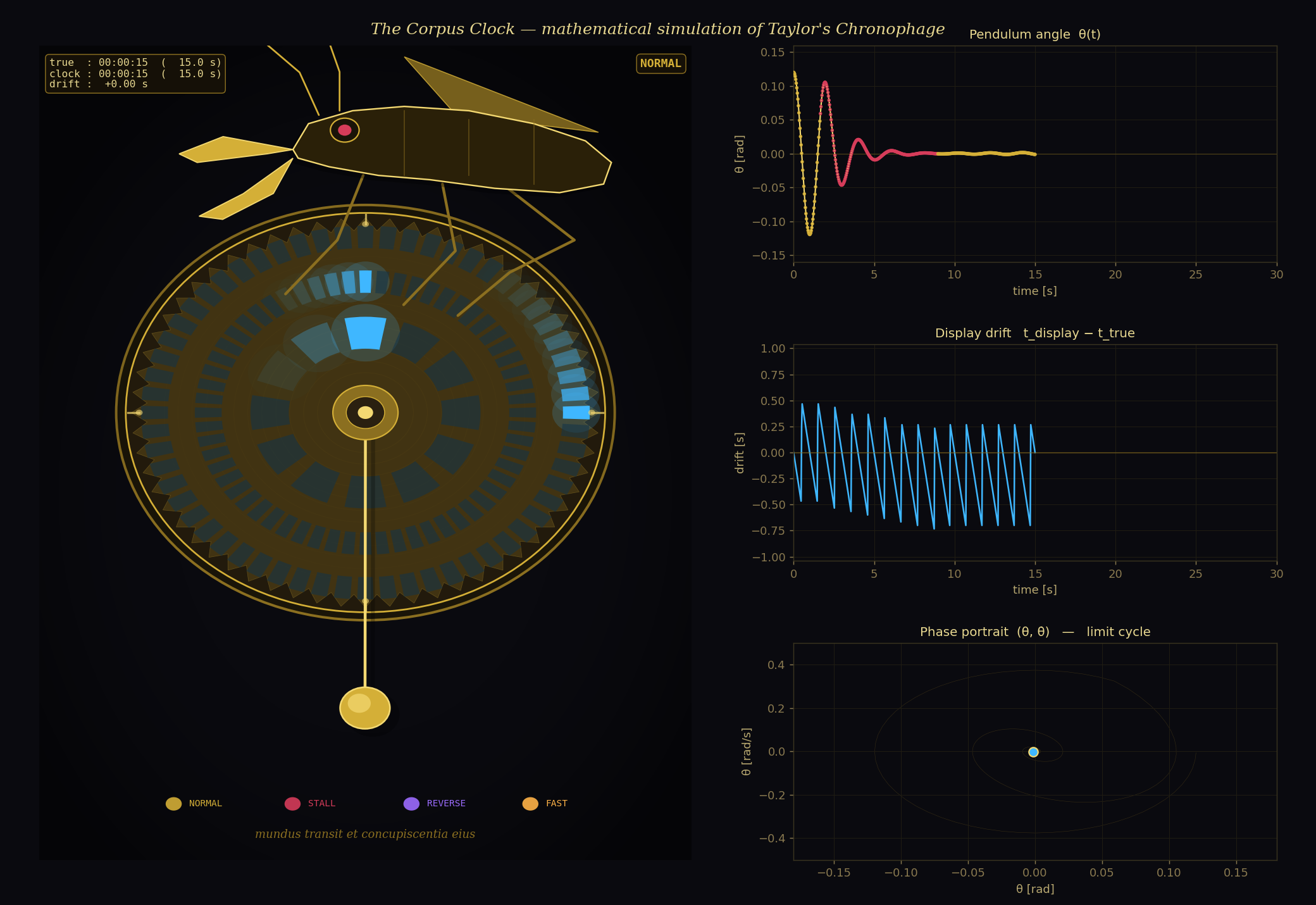
I rendered the simulation as a four-panel animated visualisation to MP4:

Left panel — The clock face: Three concentric LED rings (seconds, minutes, hours) with glowing halos and exponential-decay tails; a rotating 60-tooth escape wheel visible behind the LEDs; the Chronophage creature with articulated jaw, segmented body, animated legs and antennae, and a sinister glowing eye whose colour reflects the regulator state; the pendulum swinging below with a shadow for depth; a radial vignette and concentric ripple texture.

Upper-right — Pendulum angle θ(t): A rolling time-series window, colour-coded by regulator state (gold = NORMAL, crimson = STALL, violet = REVERSE, amber = FAST).

Middle-right — Drift plot: t_display − t_true — the accumulated time error, showing the sawtooth pattern of discrete ticks and the 5-minute correction pull-back.

Lower-right — Phase portrait (θ, θ̇): The limit cycle of the escapement-driven oscillator. During STALL the trajectory spirals inward; during FAST the cycle inflates. A state-coloured comet tail shows how the tricks perturb the oscillator.

What I Learned from the Model

The limit cycle is the heartbeat. A clock is fundamentally a limit-cycle oscillator. The escapement creates a structurally stable periodic orbit in the (θ, θ̇) phase plane — energy dissipated per cycle equals energy injected per cycle. The tricks are perturbations away from this limit cycle, and the escapement always pulls the system back.

Tricks as controlled instability. What I find elegant about Taylor’s design is that the tricks don’t break the clock — they exploit the pendulum’s natural transient dynamics. A STALL is simply removing the energy input and letting damping do its work. A REVERSE is a brief opposition impulse. A FAST is a modest gain increase. The underlying oscillator is robust enough to recover every time. The spectator sees chaos; the engineer sees a system that always returns to its attractor.

The 5-minute lock is a feedback controller. The phase-lock correction is essentially a sampled integral controller: measure the accumulated error every 300 s, apply a correction, wait. The exponential bleed-off with τ = 30 s acts as a low-pass filter, preventing visible jumps while converging well before the next sample.

A familiar pattern from bioprocess engineering. If you’ve worked with fed-batch bioreactors, this structure maps directly:

• Pendulum ODE ↔ cell growth / metabolism ODE
• Escapement impulses ↔ nutrient feed pulses
• Damping ↔ cell death / dilution
• Stochastic tricks ↔ metabolic shifts, contamination events
• Phase-lock ↔ periodic offline assay + setpoint correction
• Escape-wheel ticks ↔ cumulative product yield

Same mathematical toolbox: hybrid ODEs, impulsive inputs, stochastic disturbances, periodic discrete corrections. Different domain, same bones.

What the model doesn’t do

This model reproduces the qualitative behaviour of the Corpus Clock. It’s not an engineering replica. The main simplifications:

1. Escapement dynamics. The real grasshopper pushes the pendulum continuously — the pallets never disengage. My model applies an instantaneous impulse at each zero-crossing. This preserves the correct energy balance but doesn’t capture the continuous interaction.
2. Trick generation. The real tricks come from deterministic mechanical sequences (countwheels, cams, spring-loaded detents). My Markov chain produces statistically similar output but the mechanism is fundamentally different.
3. 5-minute correction. The real clock is entirely mechanical; my model captures the effect of the periodic resync without replicating the mechanism.
4. Display optics. The real clock uses paired rotating annular discs with a Vernier effect. My visualisation uses individually addressable LED slits — geometrically simpler.
5. Uncalibrated parameters. The pendulum length, tooth count, damping ratio, and all regulator parameters are assumed values chosen for physical plausibility. They’re not measured from the real clock.
6. Drive system. The real clock has an electrically wound spring/weight that stores energy; the grasshopper transfers energy from this drive to the pendulum. My model injects energy directly at impulses with no explicit drive train.

Running the Code

The project is two Python files:

• corpus_clock_model.py — The simulation core: parameters, RK4 integration, escapement logic, Markov regulator, and phase-lock.
• corpus_clock_animate.py — The visualisation: clock face geometry, Chronophage creature, and frame-by-frame rendering to MP4 via FFmpeg.

python3 -m venv .venv
source .venv/bin/activate
pip install numpy matplotlib

python corpus_clock_model.py   # smoke test (60 ticks in 60 s)
python corpus_clock_animate.py # render animation (requires ffmpeg)

The Corpus Clock is a remarkable object — a precision timepiece deliberately made imprecise, a philosophical statement encoded in brass and gold. Modelling it as a hybrid dynamical system let me reproduce its behaviour in silico: the steady tick of the escapement, the unpredictable wandering of the tricks, the quiet correction of the phase lock, and the Chronophage ceaselessly devouring it all. The maths is classical — damped oscillators, impulsive systems, Markov chains, sampled-data control — but the combination is unusual, and building it was a lot of fun.

mundus transit et concupiscentia eius

References

1. Wikipedia, “Corpus Clock“
2. Wikipedia, “Grasshopper escapement“
3. J. C. Taylor, “The Corpus Clock,” The Pelican (Corpus Christi College alumni magazine), Easter Term edition, pp. 20–21.
4. A. L. Rawlings, The Science of Clocks and Watches, 3rd ed. (British Horological Institute, 1993).
5. Original post by me, buymeacoffee.com/kemalyaylali/simulating-corpus-clock-a-hybrid-dynamical-systems-model-taylor-chronophage